|
Receiver- input filter and Intermodulation, a design example
All receiver inputs have the same problems: Selectivity, matching, noise matching and intermodulation. As a type for all receivers, a
FM-radio input circuit is considered and new filters are shown to enhance the receivers input.
Classical input filter
The classic FM-radio input stage is a one resonator filter followed by a low noise RF-transistor. As it is well known, the input selection
is low. Simple radios even have only a untuned input filter. Using this simple circuit a lot of intermodulation products are produced in the first transistor, simulating a lot of received channels .
Due of this, receiving a weak radiostadion is impossible. Fig. and 2 shows the typical circuit which will be improved in the following context, to reach better selection and lower IM-products.
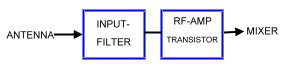 Fig 1 FM-radio input Fig 1 FM-radio input
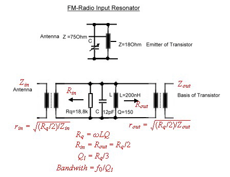
The classical resonator of Fig.2 is matched by means of coil taps which act as a real transformer. By means of this taps,
antenna and transistor are matched to the resonator from its Z to the resonator resistor, whose value is relatively low,
caused by the losses of the coil. Even worse, the loaded Q becomes very low. Practical SMD-coils in this frequency
range have a Q of about 40 to 90. The loaded Q then is only 30 and results in a minimum bandwidth of 2 to 3 Mhz.This
is five times of channel bandwidth and results in a very rough pre-election as Fig.3 shows. But that's not the only weakness
of this circuit. A unnecessary broad bandwidth increases the noise power of the input stage as the noise formula of the produced noise voltage, shows: 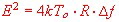
To minimize noise ,a little power mismatch has to be made. The result of this mismatch then is again a
broader bandwidth. That means realizing better selectivity would reduce the input noise too. A
additional weakness of this single resonator filter is the low attention to reject strong ratio channel intermodulation-products, outside of a tuned weak radiostadion.
Fig.2 FM-Input resonator
Fig.3 Bandwidth of classical single input-resonator
Consideration of Intermodulation
Intermodulation products are produced in transistor amplifiers due of non linearity especially in the vicinity of saturation.
Intermodulation suppression quality is defined as level distance between the products of two carriers outside band and a tuned carrier. Fig.4 may help to explain the situation in a receiver.
Fig.4 Intermodulation products
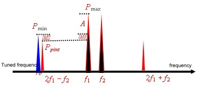 The two carries Pmax produce the products Pint. If there frequencies appear near the tuned frequency they my suppress the carrier Pmin. In difference to the
picture of Fig.4 the reality is , that the IM-products are a hedge of products which create a big power density over the total band. It is well known, that the IM
-products therefore must be 20 dB down of Pmin. This 20 db can be reached by using a proper input filter. As we can see in Fig.3, a 20 dB rejection is only reached
outside the FM-band. Therefore the level of the I-products depends only on the linearity of the first transistor-stage. Due of this, the rejection of the input filter has to be
enhanced. In this context, formulas are presented to compute the necessary filter rejection. In Fig.5, using a transistor with
an -15dB intercept point, we find 15 dB as value for the necessary filter rejection. Since no filter is ideal having a
rectangular roll-off, no filter will reach this value in the vicinity of a received channel. But each dB rejection better than the standard filter, improves the receivers quality. The two carries Pmax produce the products Pint. If there frequencies appear near the tuned frequency they my suppress the carrier Pmin. In difference to the
picture of Fig.4 the reality is , that the IM-products are a hedge of products which create a big power density over the total band. It is well known, that the IM
-products therefore must be 20 dB down of Pmin. This 20 db can be reached by using a proper input filter. As we can see in Fig.3, a 20 dB rejection is only reached
outside the FM-band. Therefore the level of the I-products depends only on the linearity of the first transistor-stage. Due of this, the rejection of the input filter has to be
enhanced. In this context, formulas are presented to compute the necessary filter rejection. In Fig.5, using a transistor with
an -15dB intercept point, we find 15 dB as value for the necessary filter rejection. Since no filter is ideal having a
rectangular roll-off, no filter will reach this value in the vicinity of a received channel. But each dB rejection better than the standard filter, improves the receivers quality.
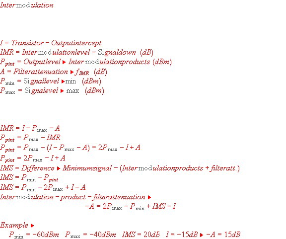 |
Fig.15 Intermodulation formulas
Lumped filter using shorted resonator
As we have seen, the filter selection depends on the Q of the used Coil. Coils in this frequency range have maximum-Q
values of about 100 .Using this value the bandwidth is still to large. A well known solution to the Q-problem is the us of
bulky helicoil resonator filters. In our case, the quarter wavelength of one resonator would be 75 cm .This is far to much.
In the following context, we propose the use of shorted wave
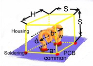
Fig.5 Shorted resonator as SMD-PCB design
resonators. We use the inductance values of this resonators as lumped circuit values to be used in lumped filters.This filters
are designed mechanically as SMD-PCB circuit. Look at Fig.5 where the arrangement is shown. Here we have the coil
soldered on two soldering eyes surrounded from the ground of the PCB. A rectangular copper sheet housing is soldered
over the coil. The other filter components are as SMD-components soldered on the other side of the PCB. The soldering
points must be carefully designed to minimize parasitc C and L. The shown dimension can be computed using the following
iteration on a pocket computer.
The shorted resonator as lumped inductance
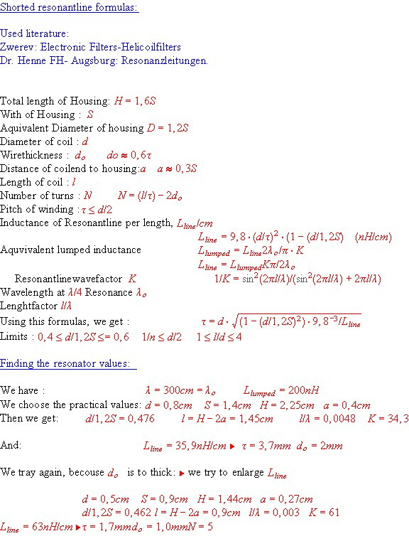
In doing so, we must know, that the value of the inductance of a shorted resonator is different from the lumped value
inductance. Formulas are given in Fig.6 to compute the necessary resonator values to realize the resonant line. Quarter
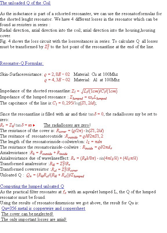
-wave resonators have Q-values up to 2000. Using the shorted resonator only leads to Q-values up to 500, and this is the
range, we need to be used for the FM-radio bandwidth. Formulas are given to find the Q of a resonator having certain
dimensions. The outcome is a unloaded Q value of 350 which then leads to an loaded Resonator resistance of 14,5k and
a bandwidth of 800 kHz for a single resonator, instead 2 MHz of Fig.2 .Fig.8 shows the formulas to compute the Q.The
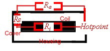
losses in the resonator are all in series as Fig.7 shows.They depend on the used skin factor of the used material. Silver or
copper material is necessary to get low Q. First we calculate the resistors due of skin effect and waves, after that we
transform it to the hot point.The Q is then found by means of the impedance of the equivalent lumped impedance and the paralleled loss resistors on the hot point.Q = Rloss / Zlumped.
Fig.6 Finding the coil values
Fig.7 The losses in the resonator Fig.8 calculation of the unloaded Q
A two resonator input filter.
As we now are able to realize a high Q-coil, it becomes possible to realize a higher order filter in the radio input. The
output of the filter must be matched either to a a 2k high-Ohm MOSFET or a 20 low-Ohm emitter input of a basis circuit
. A two resonator circuit with capacitor ground coupling was used. Using this coupling, we avoid the complicated
mechanical whole coupling of helicoil filter. We use two of the simple high-Q Coils which have no magnetic coupling at all, if properly covered. Fig.9 shows the basis circuit.
Fig.9 Basis circuit of the input filter
Fig.10 Tuning diagram
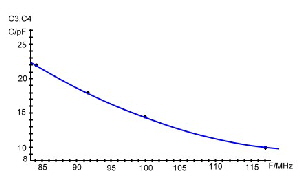
C3 and C4 are the tuning capacitors whereas C5 realizes the coupling Capacitor. It had been found, that the bandwidth is
relatively stable during frequency tuning changing C3 and C4. SMD tuning diodes can be used. Fig.10 shows the
frequency tuning diagram. Some thing must be added in the final filter circuit:
- DC-path and decoupling Capacitors for the varactors.
- SMD matching transformer to the FET.
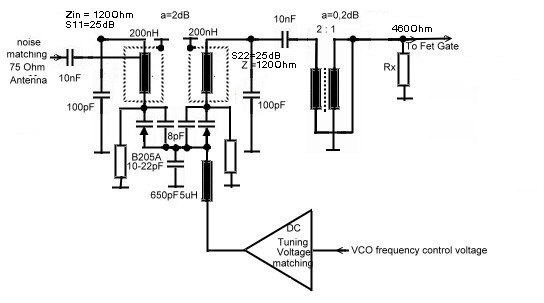
- DC-control unit to match the varactors to the VCO overall-tuning. Fig.11 shows the finally circuit.
- To match to a npn transistors emitter, the broadband transformers input and output has to be changed .This leads to
Zout = 22 Ohm
Fig.11 Two resonator Input filter of high selectivity FM-radio
Now we can consider the CAD-result of the filter in Fig. 13. We see two diagrams , one for the 1 resonator-filter of Fig
.2 and an other of the 2 resonator-filter of Fig.9 .The narrow channel bandwidth both are the same, depending only on the
loaded Q. But with the 2 resonator circuit, we have reached the goal, outsite band rejection = 15 dB at 7 Mhz distance from the tuned frequency fo.
Fig. 12 Selectivity of the two resonator filter
End of new filter---------------------------------------------------------------------------------------------------------------------------------------------
RETURN:
Improvement of simple FM-receivers input circuit using Norton-transformation
Simple receivers in the input have a untuned covering filter. The resonator of Fig.2 is shunted by means of 1k resistor to
get the necessary bandwidth. It’s clear, as Fig.13 shows, the insertion loss then is very high. With little effort, we design a
matching covering filter without the damping resistor and get a betters selectivity at less losses.
Fig.13 comparison of covering filters
Receiver input covering filter design using Norton transformation
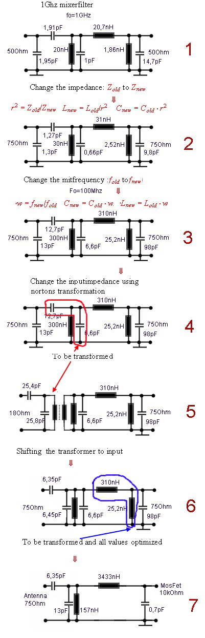
This is an example of learning filter-transformation what is done normally using computer-programs
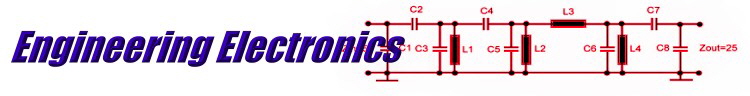
We start with a small parametric filter, which was used as output filter in a 1 Ghz mixer. (# 1). First, the impedance has to
be changed to 75 Ohm. This is done by multiplication the component values with the square of Z-ratio. (.( # 2) The next is
changing of the middle frequency by multiplication all components with the frequency factor f2 / f1. (# 3) Now we simplify
the input, by using Norton’s transformation (# 4), which adds an ideal transformer. (# 5) Now we shift the transformer to
the left side by multiplication the components on the left side of the transformer with square of Z-ratio. Removing the
transformer gets the circuit back to the 75 Ohm impedance. (# 6). Next is to transform the coils using Norton’s
transformation too. Doing so, we can remove one coil. Removing Norton’s transformer increases the output impedance
into the kOhm range, just fitting to a MOSFET gate. (#) 7. The 0.7 pf output capacitor can be gate input-Capacitor.
Antenna noise matching can be made changing the input capacitor. Comparing the results at Fig.13 with the classical filter shows, insertion loss is only half.
Fig 14 Design transformation of a untuned covering input filter
RETURN:
|